Pytorchで2値分類やってみた。
必要なライブラリをインポート
import numpy as np
import matplotlib.pyplot as plt
import torch
import torch.nn as nn
import torch.optim as optim
from torchinfo import summary
from torchviz import make_dot
import torchvision.datasets as datasets
import torchvision.transforms as transforms
from torch.utils.data import Dataset
from torch.utils.data import DataLoader
データセットを取得・構築
機械学習に使うデータセットを用意する。sklearnでダウンロード。
from sklearn.datasets import load_iris

iris = load_iris()
ダウンロードしたデータは、以下のようになっている。
{'DESCR': '.. _iris_dataset:\n\nIris plants datas ...(省略)',
 'data': array([[5.1, 3.5, 1.4, 0.2],
        [4.9, 3. , 1.4, 0.2],
        [4.7, 3.2, 1.3, 0.2],
        [4.6, 3.1, 1.5, 0.2],
        [5. , 3.6, 1.4, 0.2],
        [5.4, 3.9, 1.7, 0.4],
              (省略)
        [6.7, 3. , 5.2, 2.3],
        [6.3, 2.5, 5. , 1.9],
        [6.5, 3. , 5.2, 2. ],
        [6.2, 3.4, 5.4, 2.3],
        [5.9, 3. , 5.1, 1.8]]),
 'data_module': 'sklearn.datasets.data',
 'feature_names': ['sepal length (cm)',
                   'sepal width (cm)',
                   'petal length (cm)',
                   'petal width (cm)'],
 'filename': 'iris.csv',
 'frame': None,
 'target': array([0, 0, 0, 0, 0, 0, 0, 0, 0, 0, 0, 0, 0, 0, 0, 0, 0, 0, 0, 0, 0, 0,
        0, 0, 0, 0, 0, 0, 0, 0, 0, 0, 0, 0, 0, 0, 0, 0, 0, 0, 0, 0, 0, 0,
        0, 0, 0, 0, 0, 0, 1, 1, 1, 1, 1, 1, 1, 1, 1, 1, 1, 1, 1, 1, 1, 1,
        1, 1, 1, 1, 1, 1, 1, 1, 1, 1, 1, 1, 1, 1, 1, 1, 1, 1, 1, 1, 1, 1,
        1, 1, 1, 1, 1, 1, 1, 1, 1, 1, 1, 1, 2, 2, 2, 2, 2, 2, 2, 2, 2, 2,
        2, 2, 2, 2, 2, 2, 2, 2, 2, 2, 2, 2, 2, 2, 2, 2, 2, 2, 2, 2, 2, 2,
        2, 2, 2, 2, 2, 2, 2, 2, 2, 2, 2, 2, 2, 2, 2, 2, 2, 2]),
'target_names': array(['setosa', 'versicolor', 'virginica'], dtype='<U10')}dataに150組の特徴量['sepal length (cm)', 'sepal width (cm)', 'petal length (cm)', 'petal width (cm)']が入っている。targetにはdataがそれぞれ['setosa', 'versicolor', 'virginica']のいずれであるかが保管されている。それぞれnumpy.ndarrayである。
data, targetの最初の100個を使って2値分類をする。
inputs = iris.data[:100,:2]
labels = iris.target[:100]学習用データと検証用データに分ける。sklearnのtrain_test_splitを使える。
from sklearn.model_selection import train_test_split

train_inputs_np, test_inputs_np, train_labels_np, test_labels_np = \
  train_test_split(inputs, labels, train_size=70, test_size=30, random_state=12)
学習用データの分布を可視化してみる。
inputs0 = train_inputs_np[train_labels_np == 0]
inputs1 = train_inputs_np[train_labels_np == 1]
plt.scatter(inputs0[:,0], inputs0[:,1], marker='x', c='b', label='0 (setosa)')
plt.scatter(inputs1[:,0], inputs1[:,1], marker='o', c='k', label='1 (versicolor)')
plt.xlabel('sepal_length')
plt.ylabel('sepal_width')
plt.legend()
plt.show()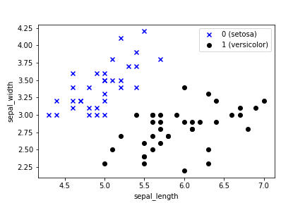
人ならこれ見ただけでスパッと分類できるね。
データをTensorに変換しておく。
train_inputs = torch.tensor(train_inputs_np).float()
train_labels = torch.tensor(train_labels_np).float().view((-1,1))
test_inputs = torch.tensor(test_inputs_np).float()
test_labels = torch.tensor(test_labels_np).float().view((-1,1))
モデル定義
2値分類ではsigmoid関数を使う。
class Net(nn.Module):
    def __init__(self, n_input, n_output):
        super().__init__()
        self.l1 = nn.Linear(n_input, n_output)
        self.sigmoid = nn.Sigmoid()

    def forward(self, x):
        x1 = self.l1(x)
        x2 = self.sigmoid(x1)
        return x2
損失関数と最適化関数定義
2値分類では損失関数として交差エントロピー関数を使う。
net = Net(2, 1)                                  # モデルインスタンス
criterion = nn.BCELoss()                         # 損失関数: 交差エントロピー関数
lr = 0.01                                        # 学習率
optimizer = optim.SGD(net.parameters(), lr=lr)   # 最適化関数: 勾配降下法
計算グラフ
とりま計算グラフを出してみる。
outputs = net(train_inputs)                                # とりま一回計算
loss = criterion(outputs, train_labels)                    # とりま一回損失計算
g = make_dot(loss, params=dict(net.named_parameters()))
display(g)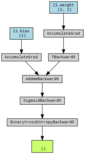
ループを回す
total_epoch = 10000                     # epoch数
log = np.zeros((0,5))                   # 損失・精度記録用
for epoch in range(total_epoch):

    # 学習フェーズ
    optimizer.zero_grad()                                               # 勾配値初期化
    train_outputs = net(train_inputs)                                   # 予測計算
    train_loss_t = criterion(train_outputs, train_labels)               # 損失計算
    train_loss_t.backward()                                             # 勾配計算
    optimizer.step()                                                    # パラメータ更新
    train_loss = train_loss_t.item()                                    # 損失の保存(スカラー値の取得)
    predicted = torch.where(train_outputs < 0.5, 0, 1)                  # 予測ラベル(1 or 0)計算
    train_acc = (predicted == train_labels).sum() / len(train_labels)   # 精度計算

    # 検証フェーズ
    with torch.no_grad():
        test_outputs = net(test_inputs)                                        # 予測計算
        test_loss_t = criterion(test_outputs, test_labels)                     # 損失計算
        test_loss =  test_loss_t.item()                                        # 損失の保存(スカラー値の取得)
        test_predicted = torch.where(test_outputs < 0.5, 0, 1)                 # 予測ラベル(1 or 0)計算
        test_acc = (test_predicted == test_labels).sum() / len(test_labels)    # 精度計算

    # 10回ごとに途中経過を記録する
    if (epoch % 10 == 0):
        print (f'Epoch [{epoch}/{total_epoch}], loss: {train_loss:.5f} acc: {train_acc:.5f} val_loss: {test_loss:.5f}, val_acc: {test_acc:.5f}')
        vals = np.array([epoch, train_loss, train_acc, test_loss, test_acc])
        log = np.vstack((log, vals))
結果
損失
plt.plot(log[:,0], log[:,1], 'b', label='train')
plt.plot(log[:,0], log[:,3], 'k', label='test')
plt.xlabel('epoch')
plt.ylabel('loss')
plt.legend()
plt.show()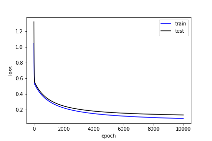
精度
plt.plot(log[:,0], log[:,2], 'b', label='train')
plt.plot(log[:,0], log[:,4], 'k', label='test')
plt.xlabel('epoch')
plt.ylabel('accuracy')
plt.legend()
plt.show()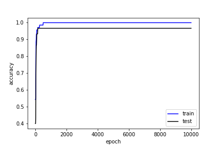
決定境界
# weight, bias出力
bias = net.l1.bias.data.numpy()
weight = net.l1.weight.data.numpy()
print(f'BIAS = {bias}, WEIGHT = {weight}')

line_x = np.array([test_inputs[:,0].min(), test_inputs[:,0].max()])
line_y = -(bias + weight[0,0] * line_x) / weight[0,1]

test_inputs0 = test_inputs_np[test_labels_np==0]
test_inputs1 = test_inputs_np[test_labels_np==1]

# 散布図
plt.scatter(test_inputs0[:,0], test_inputs0[:,1], marker='x', c='b', label='0 (setosa)')
plt.scatter(test_inputs1[:,0], test_inputs1[:,1], marker='o', c='k', label='1 (versicolor)')

# 決定境界
plt.plot(line_x, line_y, c='b')
plt.xlabel('sepal_length')
plt.ylabel('sepal_width')
plt.legend()
plt.savefig('line.png')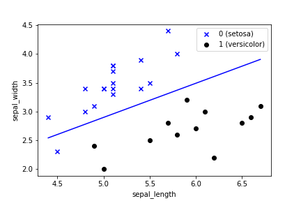
うまく分類できてるが、1つ外れてしまっている。訓練データでは精度は100%なので、もうどうしようもないが、データが100点しかないので仕方ないだろう。
決定境界の引き方は以下の通り。
データ: 、Weight:
 、バイアス:
 について、確率
 は、
は、
![\[p=\sigma(W^\mathrm{T}X+b)\]](https://blog.kiyohiroyabuuchi.com/wp-content/ql-cache/quicklatex.com-bcc2a766beab14b5106cf308e1a0aceb_l3.png "Rendered by QuickLaTeX.com")
![\[\sigma(z) = \frac{1}{1+e^{-z}}\]](https://blog.kiyohiroyabuuchi.com/wp-content/ql-cache/quicklatex.com-28a3fa73b0751a8bc2127fc7830de75e_l3.png "Rendered by QuickLaTeX.com")
確率 の時が決定境界だから、
![\[\frac{1}{2} = \sigma (W^\mathrm{T}X+b) = \frac{1}{1+e^{-(W^\mathrm{T}X+b)}}\]](https://blog.kiyohiroyabuuchi.com/wp-content/ql-cache/quicklatex.com-1e9797ce8f2a74d144444a93368305e4_l3.png "Rendered by QuickLaTeX.com")
![\[e^{-(W^\mathrm{T}X+b)} = 1\]](https://blog.kiyohiroyabuuchi.com/wp-content/ql-cache/quicklatex.com-4889137461afb0d42dacf8c3e5e77e17_l3.png "Rendered by QuickLaTeX.com")
![\[W^\mathrm{T}X+b = 0\]](https://blog.kiyohiroyabuuchi.com/wp-content/ql-cache/quicklatex.com-8ac51f485368aca78a80d957019cb0fa_l3.png "Rendered by QuickLaTeX.com")
![\[\begin{pmatrix} w_1 & w_2 \end{pmatrix} \begin{pmatrix} x_1 \\ x_2 \end{pmatrix}+b=0\]](https://blog.kiyohiroyabuuchi.com/wp-content/ql-cache/quicklatex.com-c7e3b5d03eb69c7bb81dd2e031b97b4d_l3.png "Rendered by QuickLaTeX.com")
![\[w_1 x_1 + w_2 x_2 + b = 0\]](https://blog.kiyohiroyabuuchi.com/wp-content/ql-cache/quicklatex.com-72da9c101eede73c3a02fdf8eeb5693b_l3.png "Rendered by QuickLaTeX.com")
![\[x_2 = -\frac{1}{w_2}(w_1 x_1 + b)\]](https://blog.kiyohiroyabuuchi.com/wp-content/ql-cache/quicklatex.com-3edb0a582d63e53e32125f5afcfc3e8a_l3.png "Rendered by QuickLaTeX.com")
1件のコメント